The mathematical modelling of hemodialysis can be done by making some simplifying assumptions. The first assumption is that steady-state flow exists for each of the different fluid flows: blood, dialysate, blood to dialysate, and dialysate to blood flow. Steady state means that flow rates may be different at different points in the system but that the flow rates aren’t time dependent. The other assumption is that the solute in the blood and dialysate is evenly distributed and not heavily concentrated in one area. With these assumptions in mind, Equations 1, 2, 3, and 4 were formulated. These derived equations were based off the set of two first order differential hemodialysis modeling equations in An Introduction to Fluid Mechanics, Macrocirculation, and Microcirculation, Chapter 12 [1], but with a few added flow terms and two extra variables.
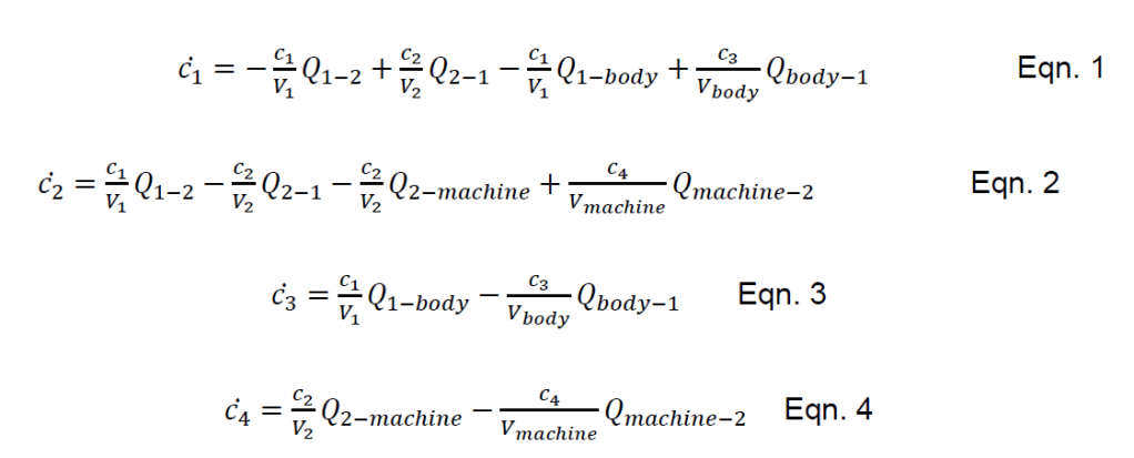
In the above equations c1 is the amount of the solute in the blood compartment of the dialyzer in units of mass; c2 is the amount of the solute in the dialysis filtrate compartment of the dialyzer in units of mass; c3 is the amount of the solute in the body of the patient in units of mass; c4 is the amount of solute in the entire dialysate solution. The variable V, in the above equations, represents the volume of either a compartment, the machine, or the human body. The subscript that follows the variable V denotes which volume is being called. The variable Q signifies the volumetric flow rate from one chamber to another and the subscript denotes the direction of the flow. Below is a diagram (Figure 1) denoting each of the variables previously described.
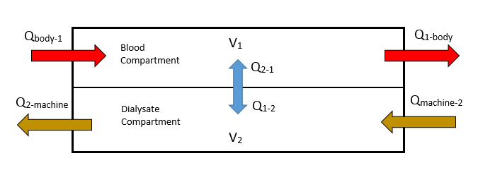
These differential equations can be solved using Laplace transforms. However, given that these equations are a set of four first order differential equations, the exact solutions would be quite extensive. To circumvent this, MATLAB’s numerical differential equation solver function, ode45, can be used. The code created to solve the set of four differential equations is found below. The initial values along with the variable values used to solve the equations can also be seen in the code. The graph (Figure 2) below shows the variance of the solute in the blood and in the dialysate with respect to time
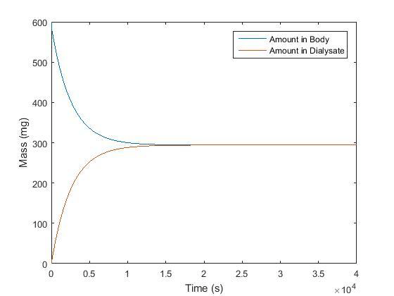
MATLAB Code
Reference
[1] Rubenstein, D. A., Frame, M. D. (2012). Biofluid mechanics: an introduction to fluid mechanics, macrocirculation, and microcirculation. Chapter 12. Amsterdam: Elsevier Academic Press.
